Spaghetti Code Dieting Tips

As an independent consultant the majority of my work is about solving novel problems faced by my clients. At a basic level, a client has a question they need answered or a problem they’d like solved and my job is to develop something that meets their needs (given the time and budget available to them).

While the novel problems I’m often presented with is part of what makes my job fun. The ad-hoc nature of each project has sometimes meant past projects were organized in an ad-hoc fashion. For some of my past analysis projects I’d output everything to a single ‘outputs’ folder and sometimes I’d just have R dump everything into the working directory. Sometimes my scripts were well documented and sometimes the names I’d used for objects made no sense.

I had developed a spaghetti ~~code~~ analysis problem.

“Spaghetti ~~code~~ [analysis] is the general term used for any ~~source code~~ [analysis] that’s hard to understand because it has no defined structure.”
Shamelessly adapted from: Orani Amroussi, “What Is Spaghetti Code and Why Is It a Problem?”, Vulcan.io

In my defense: I understand this to be a pretty common. However, being the season of new year’s resolutions I decided I needed to go on a spaghetti analysis diet. This blog post provides a summary of some of the principles that I found worked well for me:

Structuring Analysis Scripts

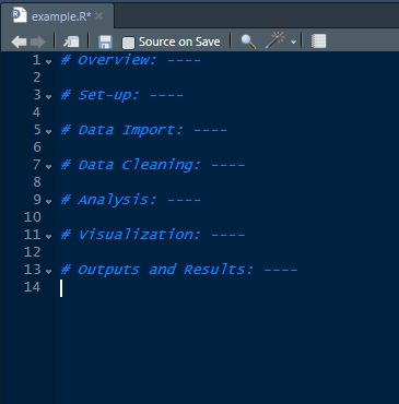
My chosen IDE when using R is Rstudio, which allows you to insert notes into your analysis scripts using ‘#’ before the text. Four hyphens (‘—-‘) can also be used to specify code sections. Although there are no hard rules for how to organize a script, I’ve found it handy to try and organize analysis across sections designed to correspond with the typical steps of an analysis project:

Overview: briefly describing the project and approach taken.
Set-up: where I load libraries and create objects for later use (such as color schemes etc).
Data Import / Cleaning: where datasets are imported and cleaned.
Analysis: for statistical tests, defining models and exploratory analysis etc.
Visualization: for producing plots.
Outputs and Results: for outputting results such as statistical summaries, simulations, datasets etc.

Depending on the complexity of your project it can also be a good idea to use separate scripts for individual steps. I typically find having separate scripts for data cleaning, analysis and visualization works well. I then have the data cleaning script output a cleaned data set that is directly used in the separate analysis and visualization scripts. This makes it easier to review specific aspects of the analysis and avoids me needing to re-run the data cleaning script unnecessarily.

Use Code Chunks to Compartmentalize Analysis

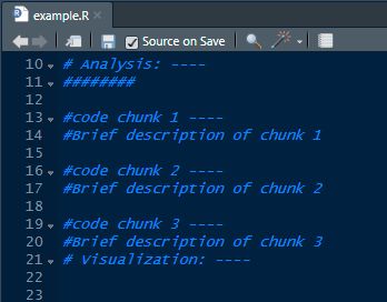
My friends in the world of Data Science noted that something that helped them produce better code was to keep projects ‘modular’. That way if a specific section of your code stopped working only that section would fail. Although this can often be hard to implement in a policy analysis environment – due to data analysis typically being structured in a sequential fashion – a happy medium I found was to group my analysis into ‘code chunks’ using Rstudio’s sections (as illustrated).

By grouping thematically similar parts of analysis together, scripts became easier to understand and unnecessary dependencies were reduced. Both because the use of code chunks encouraged better separation and ordering of individual analysis steps and as each ‘code chunk’ could be more naturally connected to the formal methodology presented to clients.

Use Documentation to Reduce the WTFs Per Minute

I’ve always invested a lot of time into documenting my code. So much so, that when completing my specialization in Data Science I was given feedback that I included too much documentation: this is feedback I’ve been happy to ignore.

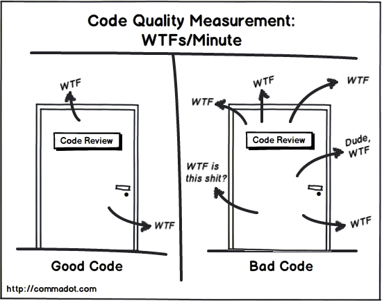
For me, documentation is about reducing the number of times I’m likely to be confused when revising old code. It should remind me what I was thinking and why I’d approached a problem in a particular way. While when working in a team, it should minimize the confused exasperation of colleagues when they’re trying to apply my model to their work.

To achieve this aim, I’ve found that when writing comments in an R analysis script it’s helpful to be as conversational and explicit as possible. In practice this means explaining what is being done, why it’s necessary and how it connects with subsequent analysis. For instance, instead of writing “This calculates the average wage by group” I might say “This calculates the average wage level by group to determine families with the lowest incomes. The results have been reshaped to a wide format to improve presentation.”

Adopt the Elements of Object Style

When searching for guidance on improving my project workflow I was a little surprised that nobody seemed to be facing the problem of being overloaded with an excessive number of confusingly named objects when conducting analysis. Clearly I was the only person in the world that was befuddled by naming structures I’d used in past projects.

My chosen strategy for addressing this was to develop an object naming ‘style guide’. Requiring that the name of an object is more explicitly related to its intended purpose using the prefixes outlined below:

For data: dta_
Temporary files: tmp_
Statistical summaries: sum_
Models (such as lm models): mod_
Custom functions: fn_
Plots and visualization: plt_
Lookup and referecne tables: lkp_
Results and Analysis: rlt_
Consistency and accuracy checks: chk_

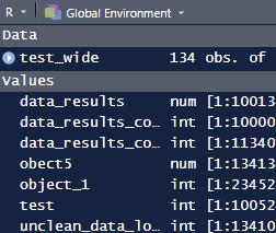
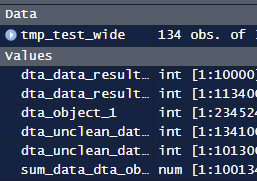
What this means in practice is that when I’m importing a dataset I might name it dta_household_income. Whereas an object with average incomes might be named ‘sum_dta_household_income_avg’. Making it clearer what the purpose of the object is and how it relates to other objects (when this is important).

Although adopting this approach completely solve the problem of poorly named objects, it has helped: as Rstudio automatically sorts objects according to its type and name. Making it easier to get a sense of what an object is designed to do (or if it can be safely deleted). Using this convention also has the added bonus of allowing the deletion of temporary objects to be deleted.

In fact, by separating my code into individual chunks and adopting this naming convention I can streamline the deletion of temporary files using the code below:

>>rm(list = ls(pattern="tmp_"))

Use Consistent Folder and File Naming Structures

One of the final habits I’ve found has helped to improve my workflow is to use a standardized setup for new analysis projects. Although this isn’t a new approach, for brevity I’ve found the following to be particularly useful:

Using R Projects for each new analysis project rather than relying on R scripts
Setting a standardized folder structure for organizing project files
Naming files thoughtfully and including dates in filenames
Disabling the project workspace being saved

Although R Projects have a number of advantages, for me the biggest advantage of switching to them has been avoiding the need to manage working directories when working on the same project on a different computer. This is because R projects automatically set the working directory to the project directory. Making it easier to work on the same project across multiple computers when using cloud-based storage services such as Dropbox.

Using a standardized folder structure for organizing analysis (or anything on a computer) is generally a good idea. However, if you work in an organization that hasn’t already implemented a standard or you work alone it can be easy to ignore. But, once you’ve created an R project setting up a rudimentary directory structure is relatively simple. For me, it typically looks like this:

Data: For storing the original input data and cleaned dataset.

Outputs: Where results of analysis are stored, such as statistical summaries.

Plots: Which is used for saving any plots generated.

Scripts: For storing individual R scripts.

Archive: Every directory includes this folder for storing old files. This is a prehistoric approach I’m yet to move away from.

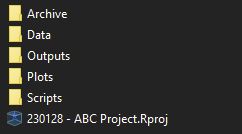
Although there is no universal standard for organizing files I’ve found this structure works well across analysis projects. In addition to the standardized structure making it easier to familiarize myself with old projects, having identical relative paths across projects makes it easier to translate old code to new projects – as the relative relative references used in the old project should remain valid for new projects.

As a side point: one approach that I’ve also found helpful is to use yyyy-mm-dd dates in all my file names. To avoid doing this manually when outputting files I have R store the current date at the start of each script. I then add the date in the filename whenever I output data, plots and statistical summaries.

>>ref_yy<-Sys.Date()

There is also a great presentation by Jennifer Bryan that covers some of important principles for naming files, which in summary says to try to make file names:

Machine readable: e.g. don’t rely on – capital letters for differentiation, spaces, and special characters and accents.
Human readable: make sure the name is intelligible
Play well with default ordering: such as starting a filename with yyyy-mm-dd ordering

Points 1 and 2 have the advantage that the metadata can be useful for later analysis. Specifically, if you use underscores or hyphens to separate specific characteristics of a file you can use this information in your analysis For instance if we have 100 files with names like ‘2012-10-14-data_envelopment_analysis-ministry_of_industry.csv” we can use the metadata to label the original source of data and/or change how the data is processed (such as only selecting data from a particular ministry).

Start From a Clean Slate

Finally, one of the first settings I change when installing Rstudio on a new computer (aside from switching to dark mode) is to disable workspace saving by default. Martin Johnsson does a good job of highlighting the reasons for this in his blog. But for me the key reason for adopting this approach is to increase the chance analysis is reproducible: meaning that if I run the script tomorrow I should get the same results as today.

By not saving your working directory you’ll be more likely to spot errors as they arise. Whether it’s a syntax error, having not loaded a necessary library as part of your script or some other software issue – regularly starting from a clean slate helps make sure any problems are presented quickly making them easier to resolve.

Finally, everybody should switch RStudio to dark mode. Dark mode is objectively better 👌 .

Some other great resources on R programming workflows:

How Should I Organize My R Research Projects?

Google’s R Style Guide

R Style Guide from the Basic R Guide for NSC Statistics